
一、blob基础
所谓Blob就是图像中一组具有某些共同属性(例如,灰度值)的连接像素。在上图中,深色连接区域是斑点,斑点检测的目的是识别并标记这些区域。OpenCV提供了一种方便的方法来检测斑点并根据不同的特征对其进行过滤。在OpenCV 3中,使用SimpleBlobDetector :: create方法创建智能指针调用该算法。
Python
Python
# Setup SimpleBlobDetector parameters.
params
=
cv2.SimpleBlobDetector_Params()
# Change thresholds
params.minThreshold
=
10
;
params.maxThreshold
=
200
;
# Filter by Area.
params.filterByArea
=
True
params.minArea
=
1500
# Filter by Circularity
params.filterByCircularity
=
True
params.minCircularity
=
0
.
1
# Filter by Convexity
params.filterByConvexity
=
True
params.minConvexity
=
0
.
87
# Filter by Inertia
params.filterByInertia
=
True
params.minInertiaRatio
=
0
.
01
# Create a detector with the parameters
ver
=
(cv2.
__version__
).split(
'.'
)
if
int
(ver[
0
])
<
3
:
detector
=
cv2.SimpleBlobDetector(params)
else
:
detector
=
C++
// Setup SimpleBlobDetector parameters.
SimpleBlobDetector
:
:Params params;
// Change thresholds
params.minThreshold
=
10;
params.maxThreshold
=
200;
// Filter by Area.
params.filterByArea
=
true;
params.minArea
=
1500;
// Filter by Circularity
params.filterByCircularity
=
true;
params.minCircularity
=
0.
1;
// Filter by Convexity
params.filterByConvexity
=
true;
params.minConvexity
=
0.
87;
// Filter by Inertia
params.filterByInertia
=
true;
params.minInertiaRatio
=
0.
01;
#
if CV_MAJOR_VERSION
<
3
// If you are using OpenCV 2
// Set up detector with params
SimpleBlobDetector detector(params);
// You can use the detector this way
// detector.detect( im, keypoints);
#
else
// Set up detector with params
Ptr
<SimpleBlobDetector
> detector
= SimpleBlobDetector
:
:create(params);
// SimpleBlobDetector::create creates a smart pointer.
// So you need to use arrow ( ->) instead of dot ( . )
// detector->detect( im, keypoints);
#
endif
二、blob参数设置
在OpenCV中实现的叫做SimpleBlobDetector,它基于以下描述的相当简单的算法,并且进一步由参数控制,具有以下步骤。
:
:Params
:
:Params()
{
thresholdStep
=
10;
//二值化的阈值步长,即公式1的t
minThreshold
=
50;
//二值化的起始阈值,即公式1的T1
maxThreshold
=
220;
//二值化的终止阈值,即公式1的T2
//重复的最小次数,只有属于灰度图像斑点的那些二值图像斑点数量大于该值时,该灰度图像斑点才被认为是特征点
minRepeatability
=
2;
//最小的斑点距离,不同二值图像的斑点间距离小于该值时,被认为是同一个位置的斑点,否则是不同位置上的斑点
minDistBetweenBlobs
=
10;
filterByColor
=
true;
//斑点颜色的限制变量
blobColor
=
0;
//表示只提取黑色斑点;如果该变量为255,表示只提取白色斑点
filterByArea
=
true;
//斑点面积的限制变量
minArea
=
25;
//斑点的最小面积
maxArea
=
5000;
//斑点的最大面积
filterByCircularity
=
false;
//斑点圆度的限制变量,默认是不限制
minCircularity
=
0.
8f;
//斑点的最小圆度
//斑点的最大圆度,所能表示的float类型的最大值
maxCircularity
= std
:
:numeric_limits
<
float
>
:
:max();
filterByInertia
=
true;
//斑点惯性率的限制变量
minInertiaRatio
=
0.
1f;
//斑点的最小惯性率
maxInertiaRatio
= std
:
:numeric_limits
<
float
>
:
:max();
//斑点的最大惯性率
filterByConvexity
=
true;
//斑点凸度的限制变量
minConvexity
=
0.
95f;
//斑点的最小凸度
maxConvexity
= std
:
:numeric_limits
<
float
>
:
:max();
//斑点的最大凸度
}
- 阈值:通过使用以minThreshold开始的阈值对源图像进行阈值处理,将源图像转换为多个二进制图像。这些阈值以thresholdStep递增,直到maxThreshold。因此,第一个阈值为minThreshold,第二个阈值为minThreshold + thresholdStep,第三个阈值为minThreshold + 2 x thresholdStep,依此类推;
- 分组:在每个二进制图像中,连接的白色像素被分组在一起。我们称这些二进制blob;
- 合并:计算二进制图像中二进制斑点的中心,并合并比minDistBetweenBlob更近的斑点;
- 中心和半径计算:计算并返回新合并的Blob的中心和半径。
并且可以进一步设置SimpleBlobDetector的参数来过滤所需的Blob类型。
按颜色:首先需要设置filterByColor =True。设置blobColor = 0可选择较暗的blob,blobColor = 255可以选择较浅的blob。按大小:可以通过设置参数filterByArea = 1以及minArea和maxArea的适当值来基于大小过滤blob。例如。设置minArea = 100将滤除所有少于100个像素的斑点。按圆度:这只是测量斑点距圆的距离。例如。正六边形的圆度比正方形高。要按圆度过滤,请设置filterByCircularity =1。然后为minCircularity和maxCircularity设置适当的值。圆度定义为(

)。圆的为圆度为1,正方形的圆度为PI/4,依此类推。

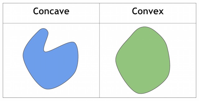
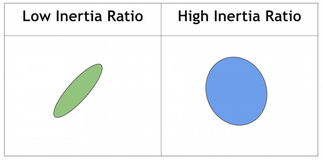
按凸性:凸度定义为(斑点的面积/凸包的面积)。现在,形状的“凸包”是最紧密的凸形,它完全包围了该形状,用不严谨的话来讲,给定二维平面上的点集,凸包就是将最外层的点连接起来构成的凸多边形,它能包含点集中所有的点。直观感受上,凸性越高则里面“奇怪的部分”越少。要按凸度过滤,需设置filterByConvexity = true,minConvexity、maxConvexity应该属于[0,1],而且maxConvexity> minConvexity。按惯性比:这个词汇比较抽象。我们需要知道Ratio可以衡量形状的伸长程度。简单来说。对于圆,此值是1,对于椭圆,它在0到1之间,对于直线,它是0。按惯性比过滤,设置filterByInertia = true,并设置minInertiaRatio、maxInertiaRatio同样属于[0,1]并且maxConvexity> minConvexity。
按凸性(左低右高)按惯性比(左低右高)


三、OpenCV的blob代码解析
在它的函数定义部分(feature2d.hpp),详细地说明了该部分代码的使用方法。

实现部分代码,来源于

单文件构成,结构比较简单,主要函数集中于detect和
findBlobs
,其他的皆为配合函数。

主要的一个数据结构,
包含了中心的位置、半径和确定性。
struct CV_EXPORTS Center
{
Point2d location;
double radius;
double confidence;
};
2.1 findblob函数实现
findblob的主要过程是寻找到当前图片的轮廓,而后根据参数中的相关定义进行筛选。其中值得注意的地方。
std::vector < std::vector<Point> > contours;
2.1.1在findContours的过程中,使用的是 RETR_LIST 和 CHAIN_APPROX_NONE
,我们来看下图

RETR_LIST
的方法是将所有的轮廓全部以链表的形式串联起来(反过来说,将丢失轮廓间的树状结构)。
2.1.2注意 轮廓遍历的大循环。进入循环后将根据参数中的每一个单项进行逐条筛选。
for (size_t contourIdx = 0; contourIdx < contours.size(); contourIdx++)
2.1.3
“面积”筛选
通过
获得moms.m00
= moments(contours[contourIdx]);
if (params.filterByArea)
{
double area = moms.m00;
if (area < params.minArea || area >
= params.maxArea)
continue;
}
这个地方调用了moments(),该函数用于计算中心矩。
设f(x,y)是一幅数字图像,
,我们把像素的坐标看成是一个二维随机变量(X, Y),那么一副灰度图可以用二维灰度图密度函数来表示,因此可以用矩来描述灰度图像的特征。

对于二值图像的来说,零阶矩M00等于它的面积,同时一阶矩计算质心/重心。OpenCV中是这样实现
bool binaryImage = false
class Moments
{
public
:
Moments();
Moments( double m00, double m10, double m01, double m20, double m11,
double m02, double m30, double m21, double m12, double m03 );
Moments( const CvMoments & moments );
operator CvMoments() const;
}
参数说明
- 输入参数:array是一幅单通道,8-bits的图像,或一个二维浮点数组(Point of Point2f)。binaryImage用来指示输出图像是否为一幅二值图像,如果是二值图像,则图像中所有非0像素看作为1进行计算。
- 输出参数:moments是一个类:
“圆度”筛选时通过来计算圆度公式,此外自带函数 arcLength 获得轮廓的周长。
double perimeter = arcLength(contours[contourIdx], true);
double ratio = 4 * CV_PI * area
/ (perimeter
*
2.1.3“颜色”筛选,只判断“圆心”的颜色。
if (params.filterByColor)
{
if (binaryImage.at <uchar > (cvRound(center.location.y), cvRound(center.location.x)) != params.blobColor)
continue;
}
这个使用方法值得商榷,在实际使用过程中不采纳。
"凸性"筛选,
if (params.filterByConvexity)
{
std : :vector < Point > hull;
convexHull(contours[contourIdx], hull);
double area = contourArea(contours[contourIdx]);
double hullArea = contourArea(hull);
if (fabs(hullArea) < DBL_EPSILON)
continue;
double ratio = area / hullArea;
if (ratio < params.minConvexity || ratio > = params.maxConvexity)
continue;
}
……
我们可以用凸度来表示斑点凹凸的程度,凸度V的定义为:

。其中,使用到了内部函数convexHull

|

|

2.1.5“惯性比”筛选,简单的来说,就是轮廓“扁”的程度。对于圆,此值是1,对于椭圆,它在0到1之间,对于直线,它是0。基本上就是取值在0-1之间,越扁越小。
if (params.filterByInertia)
{
double denominator = std : :sqrt(std : :pow( 2
* moms.mu11,
2)
+ std
:
:pow(moms.mu20
- moms.mu02,
2));
const double eps = 1e - 2;
double ratio;
if (denominator > eps)
{
double cosmin = (moms.mu20 - moms.mu02) / denominator;
double sinmin = 2 * moms.mu11 / denominator;
double cosmax = -cosmin;
double sinmax = -sinmin;
double imin = 0. 5 * (moms.mu20 + moms.mu02) -
0.
5
* (moms.mu20
- moms.mu02)
* cosmin
- moms.mu11
* sinmin;
double imax = 0. 5 * (moms.mu20 + moms.mu02) -
0.
5
* (moms.mu20
- moms.mu02)
* cosmax
- moms.mu11
* sinmax;
ratio = imin / imax;
}
else
{
ratio = 1;
}
if (ratio < params.minInertiaRatio || ratio > = params.maxInertiaRatio)
continue;
center.confidence = ratio * ratio;
}
……
二阶中心矩称为惯性矩。如果仅考虑二阶中心矩的话,则图像完全等同于一个具有确定的大小、方向和离心率,以图像质心为中心且具有恒定辐射度的椭圆。图像的协方差矩阵为:

该矩阵的两个特征值λ1和λ2对应于图像强度(即椭圆)的主轴和次轴:

而图像的方向角度θ为:

图像的惯性率I为:

这个函数定义和代码略有不同,没有进一步研究。
2.1.6特别注意“半径”的计算方法
//compute blob radius
{
std : :vector < double
> dists;
for (size_t pointIdx = 0; pointIdx < contours[contourIdx].size(); pointIdx ++)
{
Point2d pt = contours[contourIdx][pointIdx];
dists.push_back(norm(center.location - pt));
}
std : :sort(dists.begin(), dists.end());
center.radius = (dists[(dists.size() - 1) / 2] + dists[dists.size() / 2]) / 2.;
}
采用的是排序取中间值的方法,值得借鉴。
2.2 detect函数实现
2.2.1
Mat grayscaleImage;
if (image.channels() == 3 || image.channels() == 4)
cvtColor(image, grayscaleImage, COLOR_BGR2GRAY);
else
grayscaleImage = image.getMat();
if (grayscaleImage.type() != CV_8UC1) {
CV_Error(Error : :StsUnsupportedFormat, "Blob detector only supports 8-bit images!");
}
2.2.2最外层的循环采用的是遍历阈值的方法,该方法非常值得借鉴。
for ( double thresh = params.minThreshold; thresh < params.maxThreshold; thresh += params.thresholdStep)
{
Mat binarizedImage;
threshold(grayscaleImage, binarizedImage, thresh, 255, THRESH_BINARY);……
2.2.3
for ( double thresh = params.minThreshold; thresh < params.maxThreshold; thresh += params.thresholdStep)
{
Mat binarizedImage;
threshold(grayscaleImage, binarizedImage, thresh, 255, THRESH_BINARY);
std : :vector < Center > curCenters;
findBlobs(grayscaleImage, binarizedImage, curCenters);
std : :vector < std : :vector <Center > > newCenters;
for (size_t i = 0; i < curCenters.size(); i ++)
{
bool isNew = true;
for (size_t j = 0; j < centers.size(); j ++)
{
double dist = norm(centers[j][ centers[j].size() / 2 ].location - curCenters[i].location);
isNew = dist > = params.minDistBetweenBlobs && dist > = centers[j][ centers[j].size() / 2 ].radius && dist >
= curCenters[i].radius;
if ( !isNew)
{
centers[j].push_back(curCenters[i]);
size_t k = centers[j].size() - 1;
while( k > 0 && curCenters[i].radius < centers[j][k - 1].radius )
{
centers[j][k] = centers[j][k - 1];
k --;
}
centers[j][k] = curCenters[i];
break;
}
}
if (isNew)
newCenters.push_back(std : :vector <Center > ( 1, curCenters[i]));
}
std : :copy(newCenters.begin(), newCenters.end(), std : :back_inserter(centers));
}
三、一些联想
1、面积筛选这块,那个面积函数是什么意思?
面积函数是专门有实现的。
double cv::contourArea( InputArray _contour, bool oriented )


    {


        CV_INSTRUMENT_REGION();


        Mat contour = _contour.getMat();


        int npoints = contour.checkVector(2);


        int depth = contour.depth();


        CV_Assert(npoints >= 0 && (depth == CV_32F || depth == CV_32S));


        if( npoints == 0 )


            return 0.;


        double a00 = 0;


        bool is_float = depth == CV_32F;


        const Point* ptsi = contour.ptr<Point>();


        const Point2f* ptsf = contour.ptr<Point2f>();


        Point2f prev = is_float ? ptsf[npoints-1] : Point2f((float)ptsi[npoints-1].x, (float)ptsi[npoints-1].y);


        for( int i = 0; i < npoints; i++ )


        {


            Point2f p = is_float ? ptsf[i] : Point2f((float)ptsi[i].x, (float)ptsi[i].y);


            a00 += (double)prev.x * p.y - (double)prev.y * p.x;


            prev = p;


        }


        a00 *= 0.5;


        if( !oriented )


            a00 = fabs(a00);


        return a00;
但是据说,
double
area
=
moms
.
m00
;
也行,这个是为什么?
进入看看,并且删除多余的东西:
cv::Moments cv::moments( InputArray _src, bool binary )


    {


        CV_INSTRUMENT_REGION();


        const int TILE_SIZE = 32;


        MomentsInTileFunc func = 0;


        uchar nzbuf[TILE_SIZE*TILE_SIZE];


        Moments m;


        int type = _src.type(), depth = CV_MAT_DEPTH(type), cn = CV_MAT_CN(type);


        Size size = _src.size();


        if( size.width <= 0 || size.height <= 0 )


            return m;


    #ifdef HAVE_OPENCL


        CV_OCL_RUN_(type == CV_8UC1 && _src.isUMat(), ocl_moments(_src, m, binary), m);


    #endif


        Mat mat = _src.getMat();


        if( mat.checkVector(2) >= 0 && (depth == CV_32F || depth == CV_32S))


            return contourMoments(mat);


        if( cn > 1 )


            CV_Error( CV_StsBadArg, "Invalid image type (must be single-channel)" );


        CV_IPP_RUN(!binary, ipp_moments(mat, m), m);


        if( binary || depth == CV_8U )


            func = momentsInTile<uchar, int, int>;


        else if( depth == CV_16U )


            func = momentsInTile<ushort, int, int64>;


        else if( depth == CV_16S )


            func = momentsInTile<short, int, int64>;


        else if( depth == CV_32F )


            func = momentsInTile<float, double, double>;


        else if( depth == CV_64F )


            func = momentsInTile<double, double, double>;


        else


            CV_Error( CV_StsUnsupportedFormat, "" );


        Mat src0(mat);


        for( int y = 0; y < size.height; y += TILE_SIZE )


        {


            Size tileSize;


            tileSize.height = std::min(TILE_SIZE, size.height - y);


            for( int x = 0; x < size.width; x += TILE_SIZE )


            {


                tileSize.width = std::min(TILE_SIZE, size.width - x);


                Mat src(src0, cv::Rect(x, y, tileSize.width, tileSize.height));


                if( binary )


                {


                    cv::Mat tmp(tileSize, CV_8U, nzbuf);


                    cv::compare( src, 0, tmp, CV_CMP_NE );


                    src = tmp;


                }


                double mom[10];


                func( src, mom );


                if(binary)


                {


                    double s = 1./255;


                    for( int k = 0; k < 10; k++ )


                        mom[k] *= s;


                }


                double xm = x * mom[0], ym = y * mom[0];


                // accumulate moments computed in each tile


                // + m00 ( = m00' )


                m.m00 += mom[0];


                // + m10 ( = m10' + x*m00' )


                m.m10 += mom[1] + xm;


                // + m01 ( = m01' + y*m00' )


                m.m01 += mom[2] + ym;


                // + m20 ( = m20' + 2*x*m10' + x*x*m00' )


                m.m20 += mom[3] + x * (mom[1] * 2 + xm);


                // + m11 ( = m11' + x*m01' + y*m10' + x*y*m00' )


                m.m11 += mom[4] + x * (mom[2] + ym) + y * mom[1];


                // + m02 ( = m02' + 2*y*m01' + y*y*m00' )


                m.m02 += mom[5] + y * (mom[2] * 2 + ym);


                // + m30 ( = m30' + 3*x*m20' + 3*x*x*m10' + x*x*x*m00' )


                m.m30 += mom[6] + x * (3. * mom[3] + x * (3. * mom[1] + xm));


                // + m21 ( = m21' + x*(2*m11' + 2*y*m10' + x*m01' + x*y*m00') + y*m20')


                m.m21 += mom[7] + x * (2 * (mom[4] + y * mom[1]) + x * (mom[2] + ym)) + y * mom[3];


                // + m12 ( = m12' + y*(2*m11' + 2*x*m01' + y*m10' + x*y*m00') + x*m02')


                m.m12 += mom[8] + y * (2 * (mom[4] + x * mom[2]) + y * (mom[1] + xm)) + x * mom[5];


                // + m03 ( = m03' + 3*y*m02' + 3*y*y*m01' + y*y*y*m00' )


                m.m03 += mom[9] + y * (3. * mom[5] + y * (3. * mom[2] + ym));


            }


        }


        completeMomentState( &m );


        return m;


    static void momentsInTile( const Mat& img, double* moments )


    {


        Size size = img.size();


        int x, y;


        MT mom[10] = {0,0,0,0,0,0,0,0,0,0};


        MomentsInTile_SIMD<T, WT, MT> vop;


        for( y = 0; y < size.height; y++ )


        {


            const T* ptr = img.ptr<T>(y);


            WT x0 = 0, x1 = 0, x2 = 0;


            MT x3 = 0;


            x = vop(ptr, size.width, x0, x1, x2, x3);


            for( ; x < size.width; x++ )


            {


                WT p = ptr[x];


                WT xp = x * p, xxp;


                x0 += p;


                x1 += xp;


                xxp = xp * x;


                x2 += xxp;


                x3 += xxp * x;


            }


            WT py = y * x0, sy = y*y;


            mom[9] += ((MT)py) * sy;  // m03


            mom[8] += ((MT)x1) * sy;  // m12


            mom[7] += ((MT)x2) * y;  // m21


            mom[6] += x3;             // m30


            mom[5] += x0 * sy;        // m02


            mom[4] += x1 * y;         // m11


            mom[3] += x2;             // m20


            mom[2] += py;             // m01


            mom[1] += x1;             // m10


            mom[0] += x0;             // m00


        }


        for( x = 0; x < 10; x++ )


            moments[x] = (double)mom[x];
从结果来比较
Moments moms = moments(contours[contourIdx]);
double area = moms.m00;
| double area = contourArea(contours[contourIdx]);
|

|

|
是一个东西,这样的话就更应该优选contourArea,因为更具有可解释性。但是在这里,使用m00却是有道理的:

因为moms不仅在一个地方被使用,那么这次就算就是非常值的。
2、凸度的话,从结果图片上再继续分析;
凸度来表示斑点凹凸的程度,其定义为:

简单来说,比如看这张图,area(hull)>>area(contours),这个值越大,则表明原图这个尖子越多,可以表明是越复杂,越可能存在缺口,越不像一个平滑、规整的图像。
3、惯性里面有一个confidence是什么意思?
if (params.filterByInertia)


            {


                double denominator = std::sqrt(std::pow(2 * moms.mu11, 2) + std::pow(moms.mu20 - moms.mu02, 2));


                const double eps = 1e-2;


                double ratio;


                if (denominator > eps)


                {


                    double cosmin = (moms.mu20 - moms.mu02) / denominator;


                    double sinmin = 2 * moms.mu11 / denominator;


                    double cosmax = -cosmin;


                    double sinmax = -sinmin;


                    double imin = 0.5 * (moms.mu20 + moms.mu02) - 0.5 * (moms.mu20 - moms.mu02) * cosmin - moms.mu11 * sinmin;


                    double imax = 0.5 * (moms.mu20 + moms.mu02) - 0.5 * (moms.mu20 - moms.mu02) * cosmax - moms.mu11 * sinmax;


                    ratio = imin / imax;


                }


                else


                {


                    ratio = 1;


                }


                if (ratio < params.minInertiaRatio || ratio >= params.maxInertiaRatio)


                    continue;
也就是相当于:
center
.
confidence =
imin
/
imax * (
imin
/
imax)
这个来自于这里的解释:
偏心率是指某一椭圆轨道与理想圆形的偏离程度,长椭圆轨道的偏心率高,而近于圆形的轨道的偏心率低。圆形的偏心率等于0,椭圆的偏心率介于0和1之间,而偏心率等于1表示的是抛物线。直接计算斑点的偏心率较为复杂,但利用图像矩的概念计算图形的惯性率,再由惯性率计算偏心率较为方便。偏心率E和惯性率I之间的关系为:

也就是 imin / imax 越大,E越小,越解近圆。
惯性率:

偏心率:
偏心率(离心率)
偏心率(Eccentricity)是用来描述圆锥曲线轨道形状的数学量。对于圆锥曲线(二次曲线)的(不完整)统一定义:到定点(焦点)的距离与到定直线(准线)的距离的商是常数e(离心率)的点的轨迹。
当e>1时,为双曲线的一支;当e=1时,为抛物线;当0<e<1时,为椭圆;当e=0时,为一点
对于椭圆,偏心率即为两焦点间的距离(焦距,2c)和长轴长度(2a)的比值,即e=c/a。偏心率反映的是某一椭圆轨道与理想圆环的偏离程度,长椭圆轨道“偏心率”高,而近于圆形的轨道“偏心率”低。
在椭圆的标准方程 (x/a)^2+(y/b)^2=1 中,如果a>b>0焦点在X轴上,这时,a代表长轴、b代表短轴、 c代表两焦点距离的一半,有关系式 c^2=a^2-b^2,即e^2=1-(b/a)^2。因此椭圆偏心率0<e<1,短轴与长轴比值(b/a)越小,e越接近于1,椭圆也就越扁平。

4、默认参数不判断圆度,但仍体现出良好的圆的筛选。
默认情况下,是不判断圆度的,但是仍然体现出了良好的对圆的筛选。
/*


    *  SimpleBlobDetector


    */


    SimpleBlobDetector::Params::Params()


    {


        thresholdStep = 10;


        minThreshold = 50;


        maxThreshold = 220;


        minRepeatability = 2;


        minDistBetweenBlobs = 10;


        filterByColor = true;


        blobColor = 0;


        filterByArea = true;


        minArea = 25;


        maxArea = 5000;


        filterByCircularity = false;


        minCircularity = 0.8f;


        maxCircularity = std::numeric_limits<float>::max();


        filterByInertia = true;


        //minInertiaRatio = 0.6;


        minInertiaRatio = 0.1f;


        maxInertiaRatio = std::numeric_limits<float>::max();


        filterByConvexity = true;


        //minConvexity = 0.8;


        minConvexity = 0.95f;


        maxConvexity = std::numeric_limits<float>::max();
但是它的
Convexity
很高,一般来说,如果要达到这么高的
Convexity
,那么肯定是一个封闭图形;反而也可以直接使用圆度来进行判断,但是得到的结果要少一些。
5、blob和contours的区别、对比
blob和contours是高、低配关系。可以通过代码非常明显地看出,blob调用了contours方法,但仅仅是一种方法;blob在轮廓筛选这块更成熟;但contours还有一个重要的信息,那就是“轮廓间关系”。
将来在使用上,应该推广blob方法,但是可能不仅仅是调用其函数,还是需要将其内容掰开来具体研究分析;对于有“轮廓间
关系
”的情况,应该积极主动使用contours分析。
感谢阅读至此,希望有所帮助。


